RNA-seq Splicing analysis (Rinkou20210319-Wang)
1. Concept of Alternative Splicing
Alternative splicing is a process that enables a messenger RNA (mRNA) to direct synthesis of different protein variants (isoforms) that may have different cellular functions or properties.
It occurs by rearranging the pattern of intron and exon elements that are joined by splicing to alter the mRNA coding sequence.

Main types of splicing:

Or in a more detailed classification:

2. SGSeq
SGSeq provides a framework for analyzing splice events from RNA-seq data.
-R/Bioconductor package
2.1 Overview
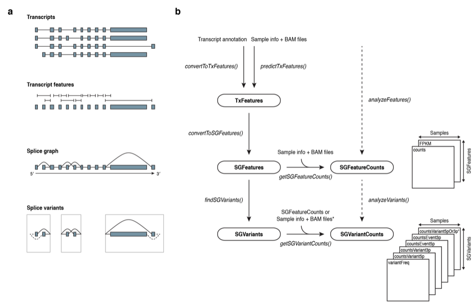 image-20210317184249496
The TxFeatures class stores discrete transcript features (exons and splice junctions) as they are observed in RNA transcripts.
From genome annotation file (.gff)
OR, de novo prediction from samples
The SGFeatures class stores features defining a splice graph (Heber et al. 2002). The splice graph is a directed acyclic (有向非巡回) graph (directed from the 5′′ end to the 3′′ end of a gene)
edges corresponding to exonic regions and splice junctions,
nodes corresponding to transcript starts, ends and splice sites.
The SGVariants class stores splice variants.
Splice variants sharing the same start and end node, together form a splice event.
=> One gene could have many splice events
one splice events is consist of many (>=2) splice variants
2.2 Preparation of Input bam files
Installation
BiocManager::install("SGSeq")
library(SGSeq)
Requirements for the Bam file:
For SGSeq to work correctly it is essential that reads were mapped with a splice-aware alignment program, such as GSNAP (T. D. Wu and Nacu 2010), HISAT (Kim, Langmead, and Salzberg 2015) or STAR (Dobin et al. 2013), which generate SAM/BAM files with custom tag ‘XS’ for spliced reads, indicating the direction of transcription.
$samtools view Rad21KD_rep1.bam |grep XS |head

HWI-D00229:285:CE888ANXX:1:2306:9926:89592	272	chr16	12360	0	19M705N47M	*0	0	CGACTTGGATCACACTCTTAGCCTCCACCACCCCGAGATCACATTTCTCACTGCCTTTTGTCTGCC	GGGGGGGGGGGGGGGGGGGGGGGGGGGGGGGGGGGGGGGGGGGGGGGGGGGGGGGGGGGGGCCCCC	NH:i:5	HI:i:5	AS:i:64	nM:i:0	NM:i:0	MD:Z:66	jM:B:c,1	jI:B:i,12379,13083	XS:A:+
HWI-D00229:285:CE888ANXX:3:1109:4408:30160	256	chr16	14482	0	30M140N36M	*0	0	CACCAGCCCCAGGTCCTTTCCCAGAGATGCCCTTGCGCCTCATGACCAGCTTGTTGAAGAGATCCG	A3AA0;>>/F</0;EG11EG1E@GB0EC1111E>1E/>F/<F11B:1:E@GGBBC:1:FGG11110	NH:i:6	HI:i:3	AS:i:66	nM:i:0	NM:i:0	MD:Z:66	jM:B:c,22	jI:B:i,14512,14651	XS:A:-
Input file.
Sample information can be stored in a data.frame or DataFrame object:
| sample_name | file_bam | paired_end | read_length | frag_length | lib_size |
|---|---|---|---|---|---|
| N1 | /xxx/bams/N1.bam | TRUE | 75 | 293 | 12405197 |
| N2 | /xxx/bams/N2.bam | TRUE | 75 | 197 | 13090179 |
| N3 | /xxx/bams/N3.bam | TRUE | 75 | 206 | 14983084 |
| N4 | /xxx/bams/N4.bam | TRUE | 75 | 207 | 15794088 |
| T1 | /xxx/bams/T1.bam | TRUE | 75 | 284 | 14345976 |
| T2 | /xxx/bams/T2.bam | TRUE | 75 | 235 | 15464168 |
| T3 | /xxx/bams/T3.bam | TRUE | 75 | 259 | 15485954 |
| T4 | /xxx/bams/T4.bam | TRUE | 75 | 247 | 15808356 |
sample_name Character vector with a unique name for each sample
file_bam Character vector or BamFileList specifying BAM files generated with a splice-aware alignment program
paired_end Logical vector indicating whether data are paired-end or single-end
read_length Numeric vector with read lengths
frag_length Numeric vector with average fragment lengths (for paired-end data)
lib_size Numeric vector with the total number of aligned reads for single-end data, or the total number of concordantly aligned read pairs for paired-end data
Prepare our own data:
bams = list.files(path = "./testbam", pattern = "*.bam$", recursive = FALSE)
labels = sub(".bam", "", bams)
bams = paste0("./testbam/", bams)
df <- data.frame(sample_name=labels, file_bam=bams)
df_full <- getBamInfo(df, cores = 32) #Obtain bam information
df_full
| sample_name | file_bam | paired_end | read_length | frag_length | lib_size |
|---|---|---|---|---|---|
| Control_rep1 | ./testbam/Control_rep1.bam | FALSE | 66 | NA | 4347199 |
| Control_rep2 | ./testbam/Control_rep2.bam | FALSE | 66 | NA | 4075464 |
| Rad21KD_rep1 | ./testbam/Rad21KD_rep1.bam | FALSE | 66 | NA | 4071598 |
| Rad21KD_rep2 | ./testbam/Rad21KD_rep2.bam | FALSE | 66 | NA | 4190821 |
2.3 Transcript annotation
2.3.1 Transcript annotation can be obtained via a TxDb object or imported from GFF format.
library(TxDb.Hsapiens.UCSC.hg38.knownGene)
txdb <- TxDb.Hsapiens.UCSC.hg38.knownGene
txdb <- keepSeqlevels(txdb, "chr16") # here we focus on chr16 for test.
!! note we have to unify the format of chromosome name:
NCBI style:
1,2,3,...orUCSC style:
chr1,chr2,chr3,...
#First check the format in bam file
> seqlevelsStyle(txdb) <- "UCSC" #change style
> seqlevels(txdb) #check
[1] "chr16"
2.3.2 Make TxFeatures objects
To work with the annotation in the SGSeq framework, transcript features are extracted from the TxDb object using function convertToTxFeatures().
txf_ucsc <- convertToTxFeatures(txdb)
head(txf_ucsc)
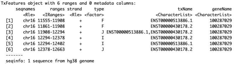 image-20210318104730709
convertToTxFeatures() returns a TxFeatures object, which is a GRanges-like object with additional columns. -
Column type indicates the feature type and can take values
J (splice junction)
I (internal exon)
F (first/5′′-terminal exon)
L (last/5′′-terminal exon)
U (unspliced transcript)
txName indicate the transcript
geneName indicate the gene
2.3.3 The splice graph and the SGFeatures class
sgf_ucsc <- convertToSGFeatures(txf_ucsc)
head(sgf_ucsc)
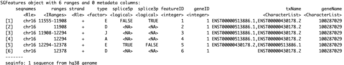 image-20210318105601948
imilar to TxFeatures, an SGFeatures object is a GRanges-like object with additional columns.
Column type for an SGFeatures object takes values
J (splice junction)
E (disjoint exon bin)
D (splice donor site)
A (splice acceptor site).
spliced5p and spliced3p indicate whether exon bins have a mandatory splice at the 5′′ and 3′′ end
visualize splicing based on annotations:
plotSpliceGraph(sgf_ucsc, geneID = 1, toscale = "exon")
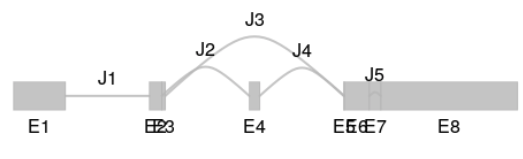 image-20210318105939156
2.4 Splice analysis on our data
2.4.1 Splice graph analysis based on annotated transcripts
sgfc_ucsc <- analyzeFeatures(df_full, features = txf_ucsc,cores = 32)
sgfc_ucsc
class: SGFeatureCounts
dim: 6 4
metadata(0):
assays(2): counts FPKM
rownames: NULL
rowData names(0):
colnames(4): Control_rep1 Control_rep2 Rad21KD_rep1 Rad21KD_rep2
colData names(6): sample_name file_bam ... frag_length lib_size
analyzeFeatures() returns an SGFeatureCounts object.
colData(sgfc_ucsc)  ##sample information as colData
rowRanges(sgfc_ucsc) ##splice graph features as rowRanges
head(counts(sgfc_ucsc)) ##counts store compatible fragment counts
head(FPKM(sgfc_ucsc)) ##FPKM store compatible FPKMs
Counts for exons and splice junctions are based on structurally compatible fragments. In the case of splice donors and acceptors, counts indicate the number of fragments with reads spanning the spliced boundary (overlapping the splice site and the flanking intronic position).
FPKM values are calculated as $(x/NL)*10^6$, where $x$ is the number of compatible fragments, $N$ is the library size (stored in lib_size) and L is the effective feature length (the number of possible positions for a compatible fragment).
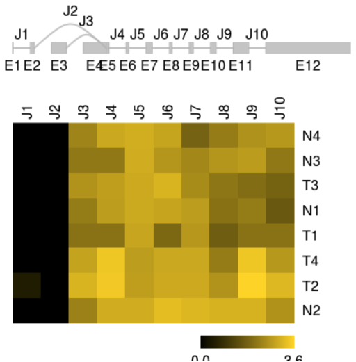
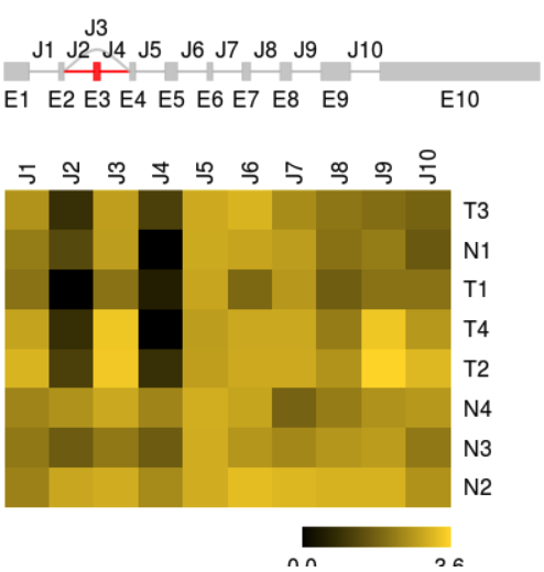
FPKMs for splice graph features can be visualized with function plotFeatures.
plotFeatures(sgfc_ucsc, geneID = 1,include = "junction",toscale="exon")
2.4.2 Splice analysis based on de novo prediction
Instead of relying on existing annotation,
annotation can be augmented with predictions from RNA-seq data.
the splice graph can be constructed from RNA-seq data without the use of annotation.
sgfc_pred <- analyzeFeatures(df_complete,cores=30)
head(rowRanges(sgfc_pred))
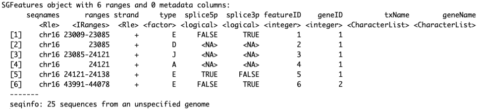 image-20210318113211055
For interpretation, predicted features can be annotated with respect to known transcripts.
The annotate() function assigns compatible transcripts to each feature and stores the corresponding transcript and gene name in columns txName and geneName, respectively.
sgfc_pred <- annotate(sgfc_pred, txf_ucsc)
head(rowRanges(sgfc_pred))
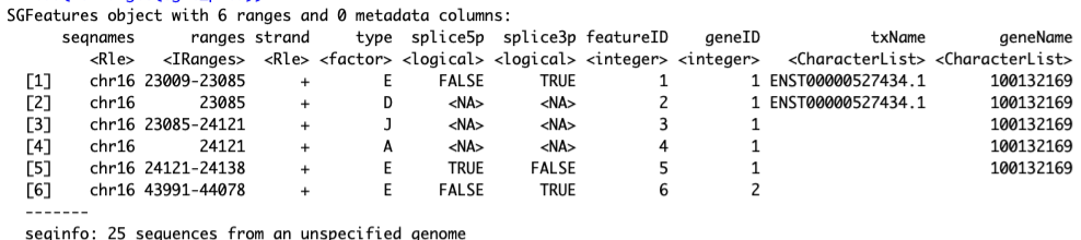 image-20210318113238805
The predicted splice graph and FPKMs can be visualized as previously.
plotFeatures(sgfc_pred, geneID =22, color_novel = "red",toscale="none",include="both")
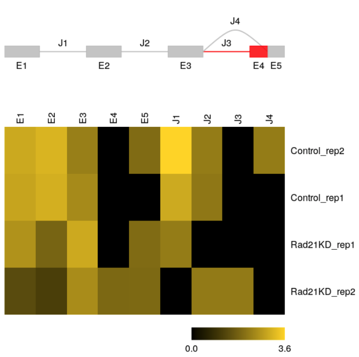
A example from SGSeq tutorial
most exons and splice junctions predicted from RNA-seq data are consistent with transcripts in the UCSC knownGene table (shown in grey)
unannotated exon (shown in red) was discovered from the RNA-seq data
predicted gene model does not include parts of the splice graph that are not expressed in the data
2.5. Splice variant identification
Instead of considering the complete splice graph of a gene, the analysis can be focused on individual splice events.
sgvc_pred <- analyzeVariants(sgfc_pred,cores=30)
sgvc_pred
class: SGVariantCounts
dim: 13504 4
metadata(0):
assays(5): countsVariant5p countsVariant3p countsEvent5p countsEvent3p variantFreq
rownames: NULL
rowData names(20): from to ... variantType variantName
colnames(4): Control_rep1 Control_rep2 Rad21KD_rep1 Rad21KD_rep2
colData names(6): sample_name file_bam ... frag_length lib_size
analyzeVariants() returns an SGVariantCounts object.
colData(sgvc_pred) ##Sample information is stored as colData
rowRanges(sgvc_pred) ##splice graph features as rowRanges
mcols(sgvc_pred) ##Information on splice variants
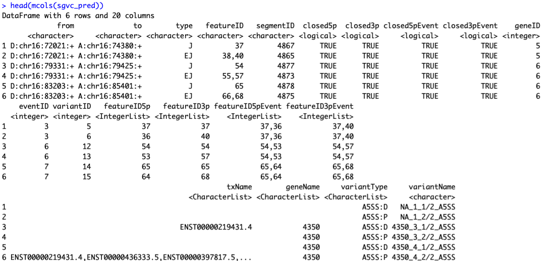 image-20210318115733817
2.6 Splice variant quantification
Splice variants are quantified locally, based on structurally compatible fragments that overlap the start or end of each variant. Local estimates of relative usage ψiψi for variant ii are obtained as the number of fragments compatible with ii divided by the number of fragments compatible with any variant belonging to the same event. For variant start SS and variant end EE ψSi=xSi/xS.ψiS=xiS/x.S and ψEi=xEi/xE.ψiE=xiE/x.E, respectively. For variants with valid estimates ψSiψiS and ψEiψiE a single estimate is calculated as a weighted mean of local estimates ψi=xS./(xS.+xE.)ψSi+xE./(xS.+xE.)ψEiψi=x.S/(x.S+x.E)ψiS+x.E/(x.S+x.E)ψiE.Estimates of relative usage can be unreliable for events with low read count. If argument min_denominator is specified for functions analyzeVariants() or getSGVariantCounts(), estimates are set to NA unless at least one of xS.x.S or xE.x.E is equal or greater to the specified value.
Estimates (0~1) of relative usage:
variantFreq(sgvc_pred)
> head(variantFreq(sgvc_pred))
     Control_rep1 Control_rep2 Rad21KD_rep1 Rad21KD_rep2
[1,]            0   0.21052632            0         0.20
[2,]            1   0.78947368            1         0.80
[3,]            0   0.80000000            0         0.40
[4,]            1   0.20000000            1         0.60
[5,]            0   0.01587302            0         0.02
[6,]            1   0.98412698            1         0.98
!! Independent of raw counts or gene expression levels
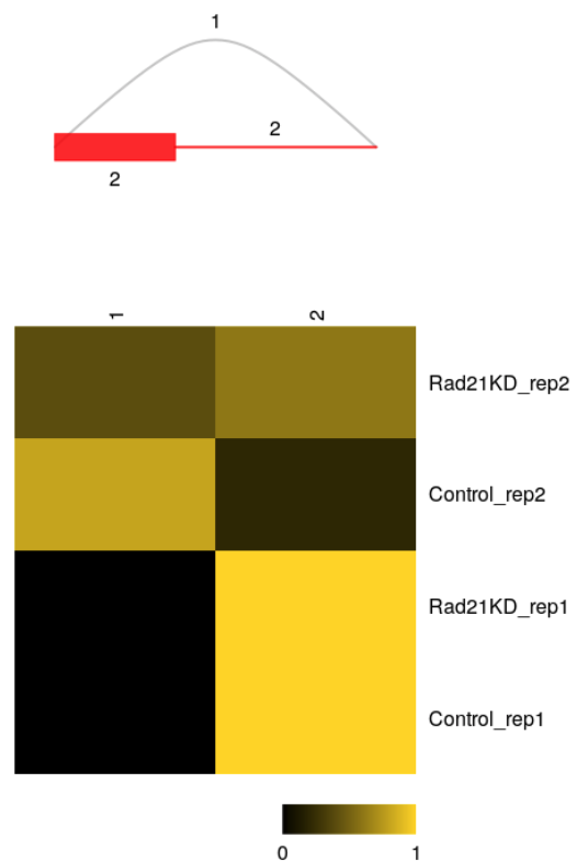
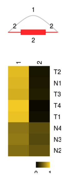
Splice variants and estimates of relative usage are visualized with function plotVariants.
plotVariants(sgvc_pred, eventID = 6, color_novel = "red",margin=0.4)
Raw counts data of each variants:
sgv <- rowRanges(sgvc_pred)
sgvc <- getSGVariantCounts(sgv, sample_info = df_full)
x <- counts(sgvc)
> head(x)
         Control_rep1 Control_rep2 Rad21KD_rep1 Rad21KD_rep2
    [1,]            0            2            0            1
    [2,]           14           15            8            8
    [3,]            0            2            0            1
    [4,]            1            1            2            2
    [5,]            0            1            0            1
    [6,]           98          114           88           84
perbase read coverages and splice junction counts can be visualized with function plotCoverage.
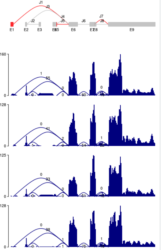 image-20210318123515875
2.7 differential splice variant
Here I tried DEXSeq (Require replicates!!)
BiocManager::install("DEXSeq")
library("DEXSeq")
x <- counts(sgvc)
vid <- as.character(variantID(sgvc))
eid <- as.character(eventID(sgvc))
sampleTable <- data.frame(row.names=c(paste("control", 1:2, sep=""), paste("cohesinKD", 1:2, sep="")), condition=rep(c("control","knockdown"), c(2, 2)))
design= ~sample+exon+condition:exon
dxd = DEXSeqDataSet(countData = x, featureID = vid,
groupID = eid, sampleData = sampleTable,
design= design)
ncpu = MulticoreParam(20)
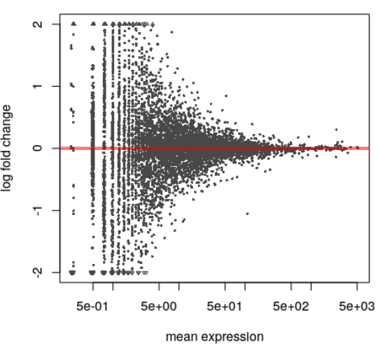
dxr <- DEXSeq(dxd,BPPARAM=ncpu)
plotMA(dxr)
2.8. Bugs
The SGSeq software did not compatiable for “alt” chromosome, so if use all chromosome:
library(TxDb.Hsapiens.UCSC.hg38.knownGene)
txdb <- TxDb.Hsapiens.UCSC.hg38.knownGene
seqlevels(txdb)

txf_ucsc <- convertToTxFeatures(txdb)
sgfc_ucsc <- analyzeFeatures(df_complete, features = txf_ucsc,cores = 32)
In these case, the chromosome include:
> seqlevels(txdb)
  [1] "chr1"                    "chr2"                    "chr3"
  [4] "chr4"                    "chr5"                    "chr6"
  [7] "chr7"                    "chr8"                    "chr9"
 [10] "chr10"                   "chr11"                   "chr12"
 [13] "chr13"                   "chr14"                   "chr15"
 [16] "chr16"                   "chr17"                   "chr18"
 [19] "chr19"                   "chr20"                   "chr21"
 [22] "chr22"                   "chrX"                    "chrY"
 [25] "chrM"                    "chr1_GL383518v1_alt"     "chr1_GL383519v1_alt"
 [28] "chr1_GL383520v2_alt"     "chr1_KI270706v1_random"  "chr1_KI270707v1_random"
 [31] "chr1_KI270708v1_random"  "chr1_KI270709v1_random"  "chr1_KI270710v1_random"
 [34] "chr1_KI270711v1_random"  "chr1_KI270712v1_random"  "chr1_KI270713v1_random"
 [37] "chr1_KI270714v1_random"  "chr1_KI270759v1_alt"     "chr1_KI270760v1_alt"
 [40] "chr1_KI270761v1_alt"     "chr1_KI270762v1_alt"     "chr1_KI270763v1_alt"
 [43] "chr1_KI270764v1_alt"     "chr1_KI270765v1_alt"     "chr1_KI270766v1_alt"
 [46] "chr1_KI270892v1_alt"     "chr1_KN196472v1_fix"     "chr1_KN196473v1_fix"
 [49] "chr1_KN196474v1_fix"     "chr1_KN538360v1_fix"     "chr1_KN538361v1_fix"
 [52] "chr1_KQ031383v1_fix"     "chr1_KQ458382v1_alt"     "chr1_KQ458383v1_alt"
 [55] "chr1_KQ458384v1_alt"     "chr1_KQ983255v1_alt"     "chr1_KV880763v1_alt"
 [58] "chr1_KZ208904v1_alt"     "chr1_KZ208905v1_alt"     "chr1_KZ208906v1_fix"
 [61] "chr1_KZ559100v1_fix"     "chr2_GL383521v1_alt"     "chr2_GL383522v1_alt"
The error will occured like:
Process features...
Obtain counts...
 validObject(.Object) でエラー:
  invalid class “RangedSummarizedExperiment” object:
    'x@assays' is not parallel to 'x'
 追加情報:  警告メッセージ:
1:  valid.GenomicRanges.seqinfo(x, suggest.trim = TRUE) で:
  GRanges object contains 11 out-of-bound ranges located on sequences chr5_KI270898v1_alt,
  chr6_KI270798v1_alt, chr12_GL383551v1_alt, chr12_GL383553v2_alt, chr12_KI270834v1_alt,
  chr17_KV766198v1_alt, chr19_GL383575v2_alt, chr19_KI270890v1_alt, chr19_KI270932v1_alt,
So, we only focus on main chromosomes by:
> txdb <- keepSeqlevels(txdb,paste0("chr",c(1:22,"X","Y","M")))
> seqlevels(txdb)
 [1] "chr1"  "chr2"  "chr3"  "chr4"  "chr5"  "chr6"  "chr7"  "chr8"  "chr9"  "chr10" "chr11" "chr12" "chr13"
[14] "chr14" "chr15" "chr16" "chr17" "chr18" "chr19" "chr20" "chr21" "chr22" "chrX"  "chrY"  "chrM"
Then, we can run the analyzeFeatures:
txf_ucsc <- convertToTxFeatures(txdb)
sgfc_pred <- analyzeFeatures(df_complete,cores=42)
sgfc_pred <- annotate(sgfc_pred, txf_ucsc)
3.MISO
![]() A pipeline of RNA-Seq samples as bowls of MISO soup (graphic by Lou Eisenman)
A pipeline of RNA-Seq samples as bowls of MISO soup (graphic by Lou Eisenman)
MISO (Mixture-of-Isoforms) is a probabilistic framework that quantitates the expression level of alternatively spliced genes from RNA-Seq data, and identifies differentially regulated isoforms or exons across samples
The MISO framework is described in Katz et. al., Analysis and design of RNA sequencing experiments for identifying isoform regulation. Nature Methods (2010).
MISO treats the expression level of a set of isoforms as a random variable and estimates a distribution over the values of this variable.
Overview:
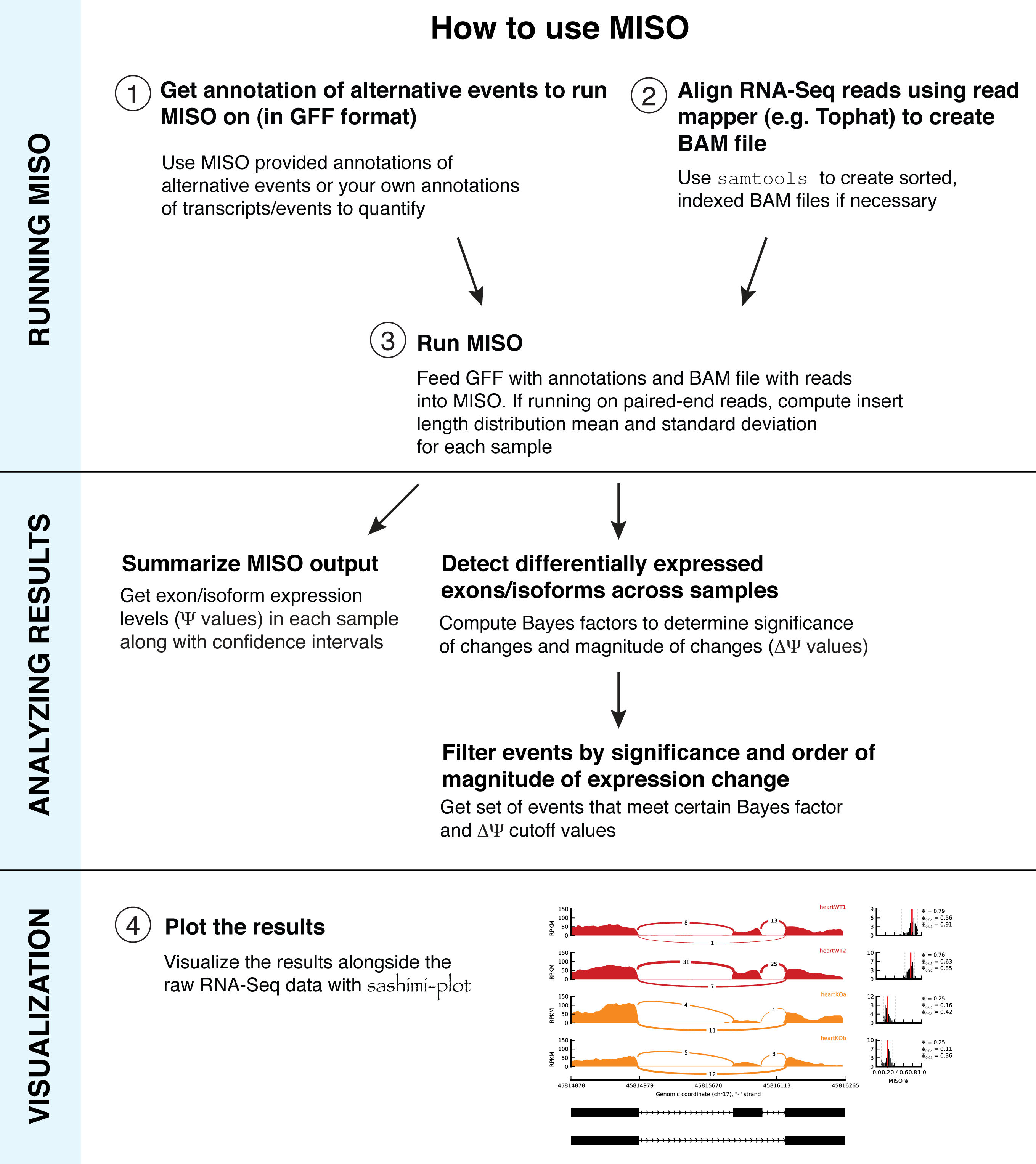 Overview of how to run MISO
3.1 Preparation
3.1.1 Installation
Miso requires Python2 !!
conda create -n py27 python=2.7
conda env list
conda activate py27
Install vis pypi
pip install misopy
3.1.2 Annotation
Two general kinds of analyses are possible:
Estimate expression level of exons (“exon-centric” analysis). Exon-centric analyses are recommended for looking at alternative splicing at the level of individual splicing events
Estimate expression level of whole transcripts (“isoform-centric” analysis). In isoform-centric analyses the expression level of whole isoforms for genes are estimated
The annotation can be in the GFF format:
which specify single alternative splicing events (“exon-centric”):
Skipped exons (SE)
Alternative 3’/5’ splice sites (A3SS, A5SS)
Mutually exclusive exons (MXE)
Retained introns (RI)
Tandem 3’ UTRs (TandemUTR)
Alternative first exons (AFE)
Alternative last exons (ALE)
chr1  SE      gene    4772649 4775821 .       -       .       ID=chr1:4775654:4775821:-@chr1:4774032:4774186:-@chr1:4772649:4772814:-;Name=chr1:4775654:4775821:-@chr1:4774032:4774186:-@chr1:4772649:4772814:-
chr1  SE      mRNA    4772649 4775821 .       -       .       ID=chr1:4775654:4775821:-@chr1:4774032:4774186:-@chr1:4772649:4772814:-.A;Parent=chr1:4775654:4775821:-@chr1:4774032:4774186:-@chr1:4772649:4772814:-
chr1  SE      mRNA    4772649 4775821 .       -       .       ID=chr1:4775654:4775821:-@chr1:4774032:4774186:-@chr1:4772649:4772814:-.B;Parent=chr1:4775654:4775821:-@chr1:4774032:4774186:-@chr1:4772649:4772814:-
chr1  SE      exon    4775654 4775821 .       -       .       ID=chr1:4775654:4775821:-@chr1:4774032:4774186:-@chr1:4772649:4772814:-.A.up;Parent=chr1:4775654:4775821:-@chr1:4774032:4774186:-@chr1:4772649:4772814:-.A
chr1  SE      exon    4774032 4774186 .       -       .       ID=chr1:4775654:4775821:-@chr1:4774032:4774186:-@chr1:4772649:4772814:-.A.se;Parent=chr1:4775654:4775821:-@chr1:4774032:4774186:-@chr1:4772649:4772814:-.A
chr1  SE      exon    4772649 4772814 .       -       .       ID=chr1:4775654:4775821:-@chr1:4774032:4774186:-@chr1:4772649:4772814:-.A.dn;Parent=chr1:4775654:4775821:-@chr1:4774032:4774186:-@chr1:4772649:4772814:-.A
chr1  SE      exon    4775654 4775821 .       -       .       ID=chr1:4775654:4775821:-@chr1:4774032:4774186:-@chr1:4772649:4772814:-.B.up;Parent=chr1:4775654:4775821:-@chr1:4774032:4774186:-@chr1:4772649:4772814:-.B
chr1  SE      exon    4772649 4772814 .       -       .       ID=chr1:4775654:4775821:-@chr1:4774032:4774186:-@chr1:4772649:4772814:-.B.dn;Parent=chr1:4775654:4775821:-@chr1:4774032:4774186:-@chr1:4772649:4772814:-.B
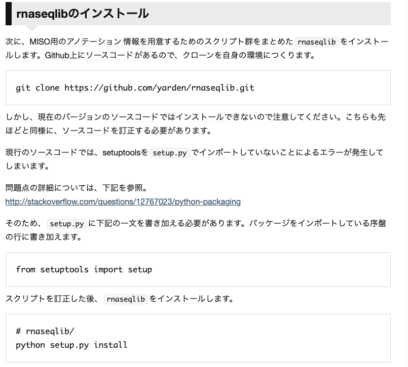
How to prepare it is introduced in a bolg (http://imamachi-n.hatenablog.com/entry/2017/03/28/234104)
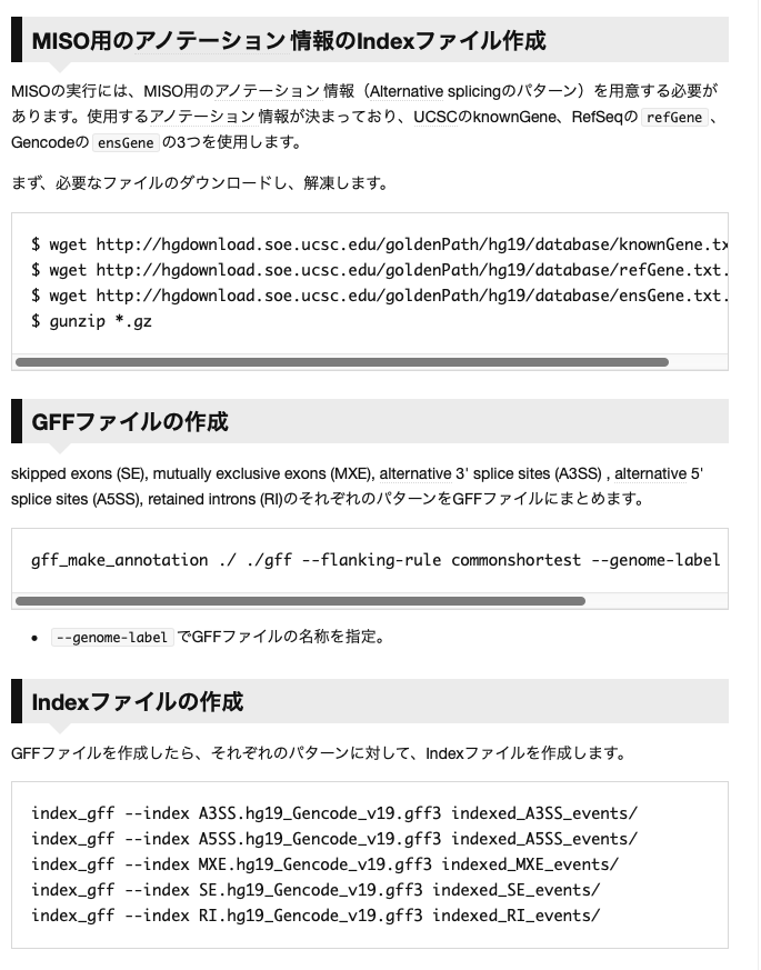
$ ls hg38_SEindex
indexed_A3SS_events
indexed_A5SS_events
indexed_MXE_events
indexed_RI_events
indexed_SE_events
Any gene models annotation can be used (e.g. from Ensembl, UCSC or RefSeq) as long as it is specified in the GFF3 format. (**“isoform-centric” **)
To estimate the expression level of whole mRNA transcripts, a GFF format containing a set of annotated transcripts for each gene can be used
3.1.3 What is Ψ values (“Percent Spliced In”. Katz et. al. 2010)
The exon-inclusion ratio, also known as percent spliced in (PSI), is a popular statistic for measuring alternative splicing events
It is defined as the ratio of the relative abundance of all isoforms containing a certain exon over the relative abundance of all isoforms of the gene containing the exon.
Ψ = PSI = splice_in / (splice_in +splice_out)。
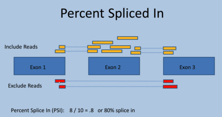 image-20210318160605839
Advantages: PSI exclusively captures a specific type of event, simple exon skipping. It also doesn’t have to rely on known transcript annotations, so can capture exon skipping events that wouldn’t be captured using other methods like the transcript ratio method.
Disadvantages: same as the advantage: it only captures exon skipping events. It wouldn’t be good at picking up switching between two totally different isoforms, alternative 3’ or 5’ ends of exons, etc. Since these complex events seem to be quite abundant, PSI will miss a lot of splice variation events.
3.2 Run Miso
for bam in `ls ~/testbam/*bam`
do
       type=SE
       prefix=`basename $bam .bam`
	     echo $prefix
	     miso --run ./hg38_SEindex $bam --output-dir misoout/${prefix}_$type -p 64 --read-len 66 #run each sample for indicated splicing types
       summarize_miso --summarize-samples misoout/$prefix.$type misomerge/$prefix.$type # merger results
done
$ ls misoout/Control_rep1_SE/
batch-genes  chr11  chr15  chr19  chr22  chr6  chrX             scripts_output
batch-logs   chr12  chr16  chr2   chr3   chr7  chrY
chr1         chr13  chr17  chr20  chr4   chr8  cluster_scripts
chr10        chr14  chr18  chr21  chr5   chr9  logs

$ ls misomerge/Control_rep1_SE/summary/
Control_rep1_SE.miso_summary
3.3 Compare samples
Compare
compare_miso --compare-samples misoout/Rad21KD_rep1_SE misoout/Contorl_rep1_SE misoCompare
$ tree misoCompare
misoCompare
└── Rad21KD_rep1_SE_vs_Control_rep1_SE
    └── bayes-factors
        └── Rad21KD_rep1_SE_vs_Control_rep1_SE.miso_bf

$ wc -l misoCompare/Rad21KD_rep1_SE_vs_Control_rep1_SE/bayes-factors/Rad21KD_rep1_SE_vs_Control_rep1_SE.miso_bf
4380
Filter
bf=/home/wang/testmiso/misoCompare/Rad21KD_rep1_SE_vs_Control_rep1_SE/bayes-factors/Rad21KD_rep1_SE_vs_Control_rep1_SE.miso_bf

filter_events --filter $bf \
      --num-inc 1 \
      --num-exc 1 \
      --num-sum-inc-exc 10 \
      --delta-psi 0.20 \
      --bayes-factor 10 \
      --output-dir ./filter_out
$ ls filter_out/
Rad21KD_rep1_SE_vs_Control_rep1_SE.miso_bf.filtered

$ wc -l Rad21KD_rep1_SE_vs_Control_rep1_SE.miso_bf.filtered
16
 Book1 - Excel 2017-03-28 22.35.39.png (38.0 kB)
details: https://miso.readthedocs.io/en/fastmiso/#detecting-differentially-expressed-isoforms
3.4 Visualization
 sashimi_plot: a tool for visualizing raw RNA-Seq data and MISO output
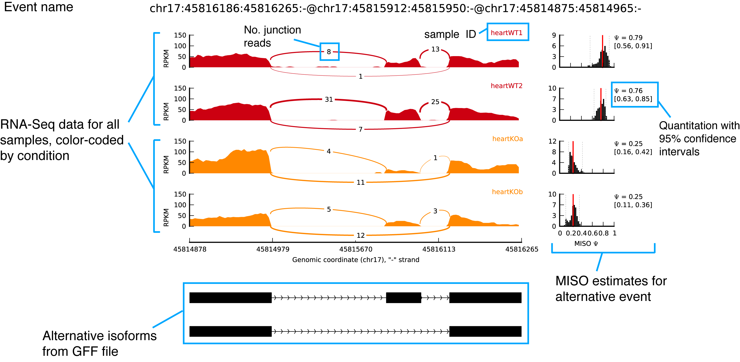 sashimi_plot example with annotations
prepare
sashimi_plot_settings.txt:[data] # directory where BAM files are bam_prefix = ~/CHX_sakata/testbam/ # directory where MISO output is miso_prefix = ./misoout/ bam_files = [ "Control_rep1.bam", "Control_rep2.bam", "Rad21KD_rep1.bam", "Rad21KD_rep2.bam"] miso_files = [ "Control_rep1.SE", "Control_rep2.SE", "Rad21KD_rep1.SE", "Rad21KD_rep2.SE"] [plotting] # Dimensions of figure to be plotted (in inches) fig_width = 7 fig_height = 5 # Factor to scale down introns and exons by intron_scale = 30 exon_scale = 4 # Whether to use a log scale or not when plotting logged = False font_size = 6 # Max y-axis ymax = 50 # Whether to plot posterior distributions inferred by MISO show_posteriors = True # Whether to show posterior distributions as bar summaries bar_posteriors = False # Whether to plot the number of reads in each junction number_junctions = True resolution = .5 posterior_bins = 40 gene_posterior_ratio = 5 # List of colors for read denisites of each sample colors = [ "#CC0011", "#CC0011", "#FF8800", "#FF8800"] # Number of mapped reads in each sample # (Used to normalize the read density for RPKM calculation) coverages = [ 36895920, 34846039, 35664259, 36249469] # Bar color for Bayes factor distribution # plots (--plot-bf-dist) # Paint them blue bar_color = "b" # Bayes factors thresholds to use for --plot-bf-dist bf_thresholds = [0, 1, 2, 5, 10, 20]
plot
for event in `cat filter_out/Rad21KD_rep1_SE_vs_Control_rep1_SE.miso_bf.filtered | cut -f1`
do
        sashimi_plot --plot-event "$event" ./hg38_SEindex \
                sashimi_plot_settings.txt --output-dir plot/
done
check results:
$ ls plot/
chr16:14644274:14644609:+@chr16:14649804:14649973:+@chr16:14655066:14655210:+.pdf
chr16:16333647:16333884:+@chr16:16336052:16336137:+@chr16:16340306:16340434:+.pdf
chr16:3283491:3284205:+@chr16:3288454:3288570:+@chr16:3289393:3291460:+.pdf
chr16:47109483:47109711:-@chr16:47086226:47086339:-@chr16:47077703:47083801:-.pdf
chr16:5097644:5097820:-@chr16:5097280:5097353:-@chr16:5095452:5095514:-.pdf
chr16:68232577:68232687:-@chr16:68232371:68232503:-@chr16:68232246:68232288:-.pdf
chr16:68533698:68533855:+@chr16:68539758:68539825:+@chr16:68557998:68558124:+.pdf
chr17:42017340:42017439:-@chr17:42003359:42003557:-@chr17:42000482:42000570:-.pdf
chr17:75978534:75978693:-@chr17:75973625:75973785:-@chr17:75957459:75957566:-.pdf
chr17:76091143:76091235:-@chr17:76090329:76090397:-@chr17:76089175:76089320:-.pdf
chr17:76094414:76094581:-@chr17:76090329:76090397:-@chr17:76089175:76089320:-.pdf
chr17:7907353:7907488:+@chr17:7907601:7907702:+@chr17:7907894:7908019:+.pdf
chr17:80415650:80415821:+@chr17:80417781:80417945:+@chr17:80423520:80423632:+.pdf
chr17:81445354:81445681:+@chr17:81446738:81446830:+@chr17:81447036:81447848:+.pdf
chr17:8460009:8460160:+@chr17:8463320:8463354:+@chr17:8466930:8468163:+.pdf
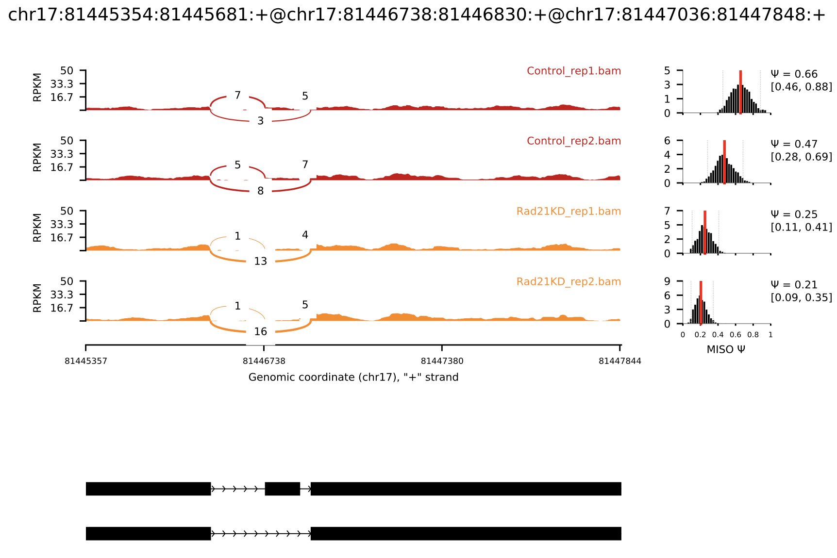 image-20210318154651195
4. Compare of MISO and DEXseq
http://imamachi-n.hatenablog.com/entry/2017/03/28/234104
MISO
最も引用数が多く、精度も高い(個人的な意見です)。Alternative splicingの解析では、デファクトスタンダードのソフト。
skipped exons (SE), mutually exclusive exons (MXE), alternative 3’ splice sites (A3SS) , alternative 5’ splice sites (A5SS), retained introns (RI)のパターンごとに解析してくれる。
n=1のデータしか扱えない(n=2同士のデータを比較することができない)。
扱えるアノテーション情報が限定されている(UCSC gene, RefSeq, Gencodeの組み合わせ。UCSCgenome browserにアップロードされている最新のデータにしか対応していない)。
結果ファイルの中身がSplicingのイベントごとに評価されているため、どの遺伝子でSplicingのパターンの変化が起こっているかわかりにくい。
p-valueによる有意差検定でなく、Bayes factorを計算しているので、どこでThresholdを引いたらいいかわかりにくい。